
We have received several inquiries about depositing RNA-seq data generated by WashU’s Genome Technology Access Center (GTAC) into the Gene Expression Omnibus (GEO) repository managed by the National Center for Biotechnology Information (NCBI). As a result, it is a good time to write a blog article providing guidance on this issue for researchers on campus. This article will be focused on the practical aspects of sharing RNA-seq data in this way. I will write more articles in the future discussing the theoretical side of Next-Generation-Sequencing (NGS) data sharing.
I would like to thank Dr. Keith Hruska and Dr. Matthew Williams for allowing me to use their RNA-seq data as an illustration example for this article. The GEO Accession Number for the dataset is GSE255815, and the primary article associated with this GEO dataset was published in the American Journal of Physiology-Renal Physiology titled as “In chronic kidney disease altered cardiac metabolism precedes cardiac hypertrophy” (https://doi.org/10.1152/ajprenal.00416.2023).
After the sequencing run, GTAC provided a standard analysis package to Dr. Hruska’s group as displayed in Figure 1. One question that comes to us often is around which files should be submitted from the package from GTAC. The short answer is that GEO formally requires two data types for submission – raw FASTQ files and processed data files containing raw and/or normalized counts (FPKM, TPM, etc.) of sequencing reads for genes and/or transcripts.
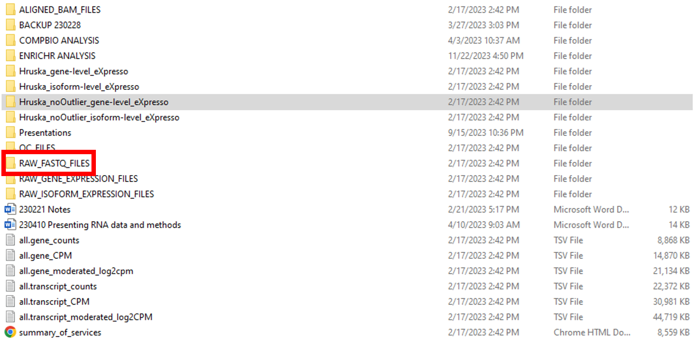
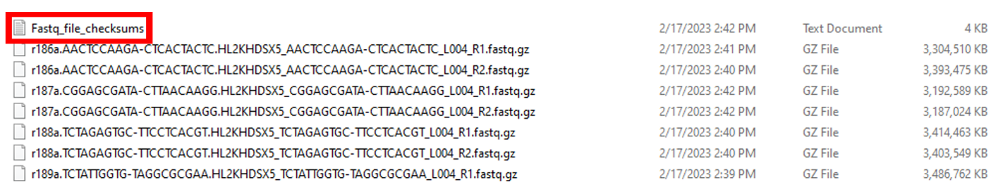
In our example, the raw FASTQ files (in the compressed fastq.gz format) are located in the RAW_FASTQ_FILES folder. The top portion of the RAW_FASTQ_FILES folder is shown in Figure 2. The first item in the folder is an MD5 checksum file. A checksum is a small-sized block of data derived from another block of digital data for the purpose of detecting errors that may have been introduced during its transmission or storage. This file is very useful as GEO strongly recommends that submitters provide MD5 checksums for raw data files. Since paired-end sequencing was used for this project, each sample has two FASTQ files – R1 for the forward read and R2 for the reverse read. The sample name is at the beginning of the file name, followed by the Illumina Library Index associated with each sequencing run.
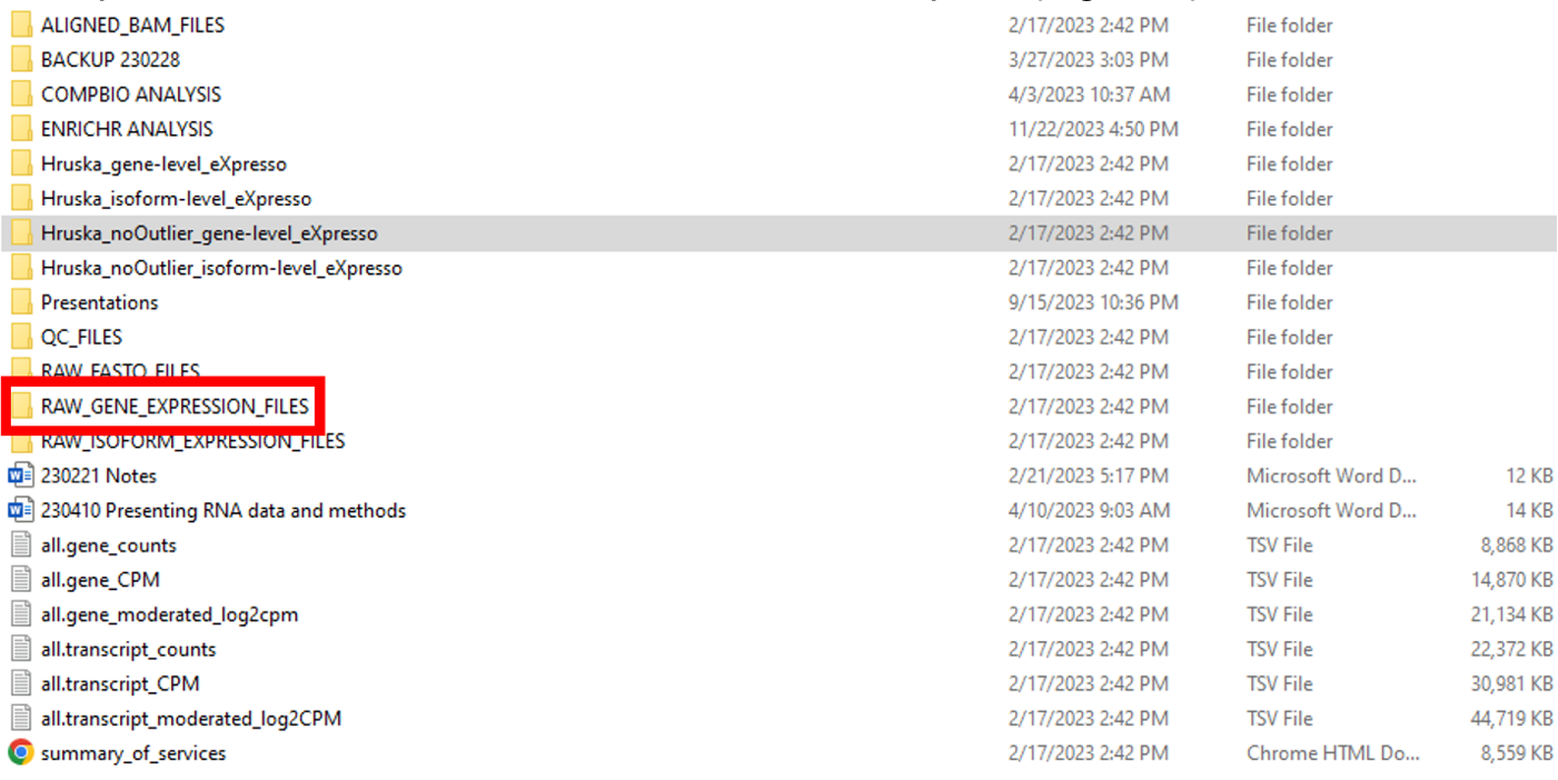
The processed data is located in a folder named RAW_GENE_EXPRESSION_FILES in the top-level folder, which contains individual-level reports (Figure 3).
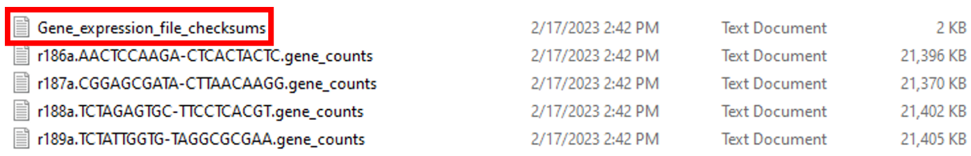
The RAW_GENE_EXPRESSION_FILES folder contains an MD5 checksum file at the top (Figure 4). Although GEO does not specifically mention checksums for processed files, many researchers choose to submit them along with checksums for raw data files. The gene counts of each sample are reported in separate text files. The names of the gene counts files follow the same format as the raw FASTQ files.
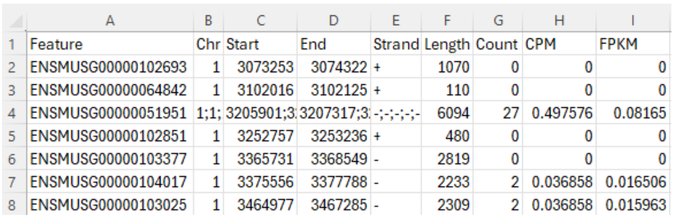
Let’s download the “gene counts” file for Sample GSM8080474 through this link from GEO, which is the second file in Figure 4. This “gene counts” file contains 9 columns, as shown in Figure 5. The first column, “Feature”, is the Ensembl stable ID for each gene. Stable IDs are created in the form ENS[species prefix][feature type prefix][a unique eleven-digit number]. For example, ENSMUSG is the prefix of a mouse gene, where MUS is the species prefix for “mouse”, and G is the feature type prefix for “gene”. The next five columns provide genomic coordination information of a gene: chromosome number, start and end base position, strand orientation, and full transcript length. The last three columns provide gene expression data: raw counts, counts per million (CPM) and Fragments Per Kilobase Million (FPKM). This blog article is a good read to understand these numbers. The total number of gene features reported in this file is 55,487.
So far, we have described two data types that can be used for GEO submission. However, there is an alternative set of processed data files that can be submitted to GEO along with the raw FASTQ files. Going back to the top-level folder, there are six TSV files in the top-level folder (“all.gene_counts”, “all.gene_CPM”, “all.gene_moderated_log2cpm”, “all.transcript_counts”, “all.transcript_CPM”, “all.transcript_moderated_log2CPM’) (Figure 6). These processed data files contain expression data at the whole study level, instead of the individual sample level.

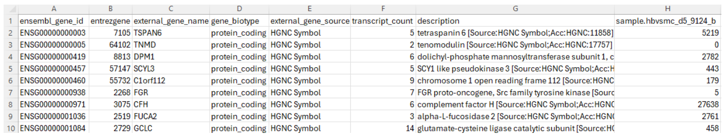
Some researchers prefer to submit study-level processed data files instead of sample-level processed data files. In our example, Dr. Hruska’s team decided to submit sample-level processed data files. In order to demonstrate the content of study-level processed data files, we are going to look at another dataset GSE283004. In this dataset, there is one study-level processed file titled “GSE283004_Fig_2-3_Somatic_RNA-seq_all.gene_counts.tsv.gz”, which can be downloaded through this link. This file contains gene expression counts for 55,209 genes across 20 biological samples (Figure 7). The first three columns correspond to the “Ensembl stable ID” for a gene, “Entrez Gene ID” for a gene (more information in this reference) and the gene name mostly from the HUGO Gene Nomenclature Committee (HGNC). The fourth column specifies gene types. The most common type is “protein coding”. Other types include “rRNA”, “SnoRNA”, “SnRNA”, “miRNA”, “lincRNA”, “scaRNA”, “antisense”, several pseudogene types, IgG and T cell receptor genes, and other minor types. The fifth column provides the resources of gene names. Besides “HGNC”, the other resources are “Clone-based (Ensembl) gene”, “RNA families database (Rfam)”, “NCBI gene database”, and “miRbase”. The sixth column specifies the number of splicing variants used in the calculation. The seventh column provides a concise description for a gene. The next 20 columns provide the gene expression counts in the 20 samples in this dataset, as each column contains data from one sample. For clarity, Figure 7 only shows the first column (Column H) of gene expression count for the first sample.
There are pros and cons for these two report formats. The individual-level reports contain more information and can be more easily used for bioinformatics analysis. However, individual-level reports cannot be used readily for cross-sample comparison. The study-level reports are easier for comparison between samples and are more intuitive to use. However, they only contain either raw counts or CPM, but not both. I did a quick survey of GEO datasets deposited by WashU researchers, and I found that most researchers deposited individual-level data to GEO in the last year.
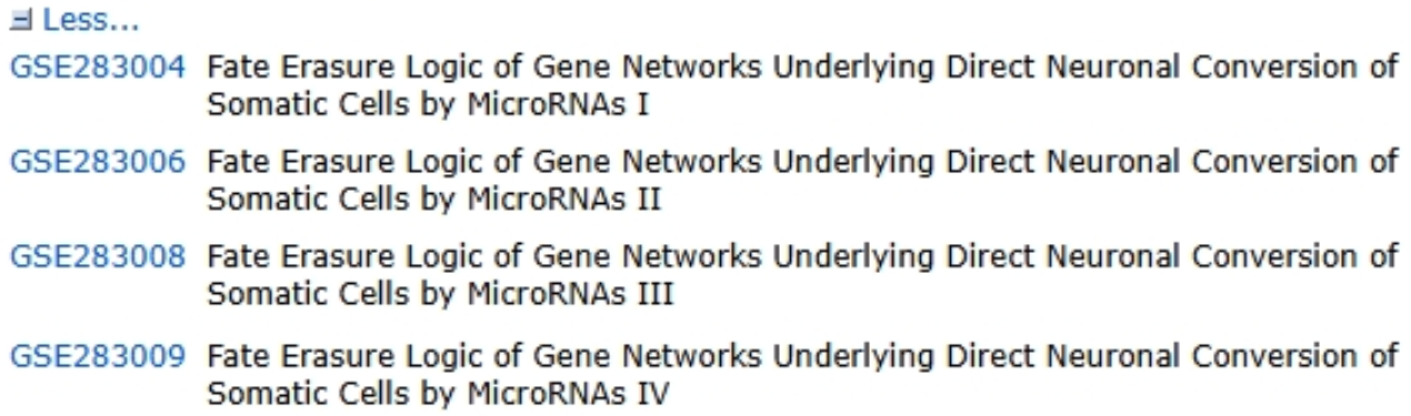
Finally, I would like to introduce the concept of “SubSeries” and “SuperSeries”. In many complex biomedical studies, researchers will perform many RNA-seq experiments. If the dataset is big, it may be a good idea to split data into multiple datasets according to experimental conditions (“SubSeries”), and group them together under a GEO “SuperSeries”. For example, our previous dataset GSE283004 is a “SubSeries” of a SuperSeries GSE283010. This SuperSeries GSE283010 includes metadata of a big research study with 66 biological samples, but itself does not contain any processed data files. Instead, the processed data files in this study are submitted into four Subseries under this SuperSeries: GSE283004, GSE283006, GSE283008 and GSE283009 (Figure 8). Each SubSeries contains data for a separate section of the primary publication. Although in this example, researchers only submitted study-level processed data files, it is possible to submit sample-level processed data files in each SubSeries.
In this article, I shared a few tips about data files during the RNA-seq data submission process. In a future article, I will discuss the metadata spreadsheet used by GEO. If you need help submitting genomic data, please do not hesitate to contact me at jianx@wustl.edu or the Becker Data Management and Sharing Team at BeckerDMS@wustl.edu.